Toy Example#
[1]:
import scanpy as sc
import singleCellHaystack as hs

sc.set_figure_params(facecolor="white", dpi=90)
Load toy data#
[2]:
adata = hs.load_toy()
adata
[2]:
AnnData object with n_obs × n_vars = 601 × 500
    obsm: 'X_tsne'
[3]:
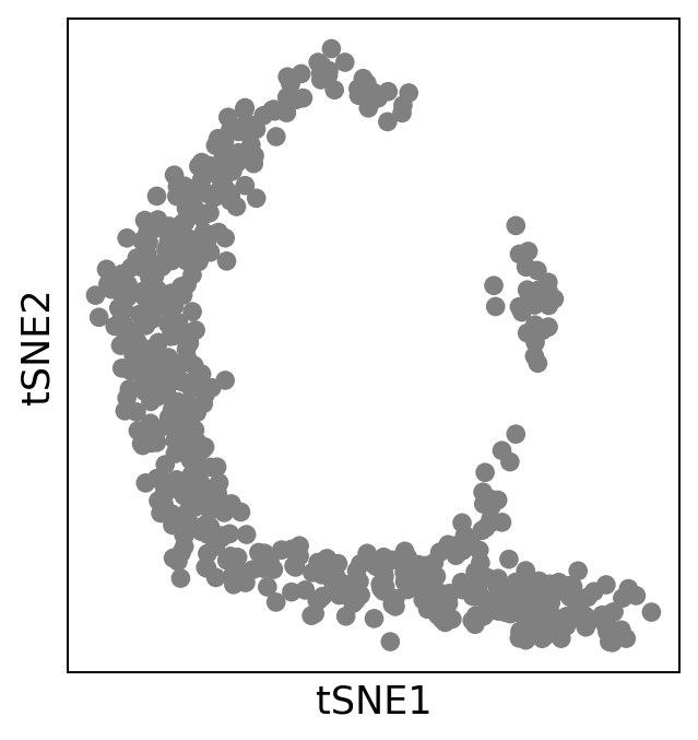
sc.pl.scatter(adata, basis="tsne")
Run haystack#
[4]:
res = hs.haystack(adata, coord="tsne", n_randomizations=100, n_genes_to_randomize=100, spline_method="ns")
> starting haystack ...
> entering array method ...
> scaling coordinates ...
> calculating feature stds ...
> calculating grid points ...
> calculating distance to cells ...
> calculating densities ...
> calculating Q dist ...
> calculating KLD for 500 features ...
100%|███████████████████████████████████████████████████████████████████████████████| 500/500 [00:00<00:00, 7301.81it/s]
> calculating feature's CV ...
> selecting genes to randomize ...
> calculating randomized KLD ...
100%|█████████████████████████████████████████████████████████████████████████████████| 100/100 [00:01<00:00, 81.12it/s]
> calculating P values ...
> done.
QC#
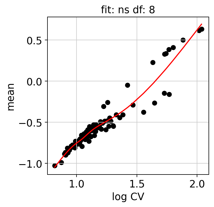
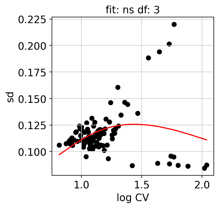
We can examine some of the QC plots. First the randomization fits. These are used to calculate KLD from randomized expression levels for a subset of genes, in order to estimate the values to the entire gene set.
[5]:
hs.plot_rand_fit(res, "mean")
hs.plot_rand_fit(res, "sd")
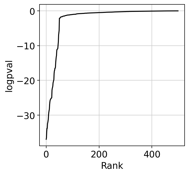
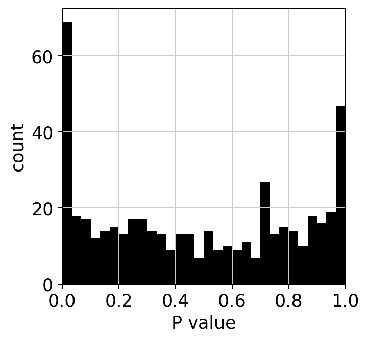
The ranking of logpval and distribution of pval gives us some idea of how many significant genes we can detect.
[6]:
hs.plot_pval_rank(res)
hs.plot_pval_hist(res)
Results#
A pandas DataFrame with the results can be obtained. By default the results are sorted by logpval_adj.
[7]:
import pandas as pd
[8]:
sum = res.top_features(10)
sum
[8]:
| gene | KLD | CV | pval | pval_adj | logpval | logpval_adj | |
|---|---|---|---|---|---|---|---|
| 241 | gene_242 | 1.738191 | 2.627666 | 1.066598e-37 | 5.332992e-35 | -36.971999 | -34.273029 |
| 338 | gene_339 | 1.861424 | 2.718406 | 2.894843e-37 | 1.447422e-34 | -36.538375 | -33.839405 |
| 496 | gene_497 | 2.007779 | 2.860687 | 1.749626e-35 | 8.748131e-33 | -34.757055 | -32.058085 |
| 274 | gene_275 | 1.733409 | 2.698842 | 1.510932e-34 | 7.554659e-32 | -33.820755 | -31.121785 |
| 350 | gene_351 | 1.849559 | 2.781079 | 1.538332e-34 | 7.691660e-32 | -33.812950 | -31.113980 |
| 61 | gene_62 | 2.027718 | 2.931154 | 3.283019e-33 | 1.641509e-30 | -32.483727 | -29.784757 |
| 136 | gene_137 | 1.791516 | 2.784830 | 6.520173e-33 | 3.260087e-30 | -32.185741 | -29.486771 |
| 316 | gene_317 | 1.762123 | 2.776867 | 1.982998e-32 | 9.914989e-30 | -31.702678 | -29.003708 |
| 243 | gene_244 | 1.664939 | 2.719325 | 7.226574e-32 | 3.613287e-29 | -31.141068 | -28.442098 |
| 78 | gene_79 | 2.238983 | 3.174348 | 1.517525e-30 | 7.587625e-28 | -29.818864 | -27.119894 |
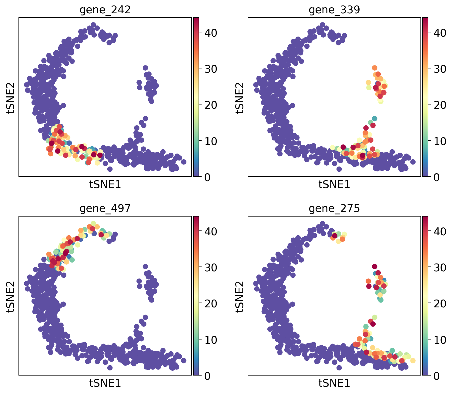
Plot top 4 genes.
[9]:
sc.pl.tsne(adata, color=sum.gene.iloc[:4], ncols=2, cmap="Spectral_r")
Export results#
[10]:
#sum.to_csv("toy-results.tsv")