Single Cell Transcriptomics (PBMC3k)#

[1]:

import scanpy as sc
import singleCellHaystack as hs

sc.set_figure_params(facecolor="white", dpi=90)

Load data#

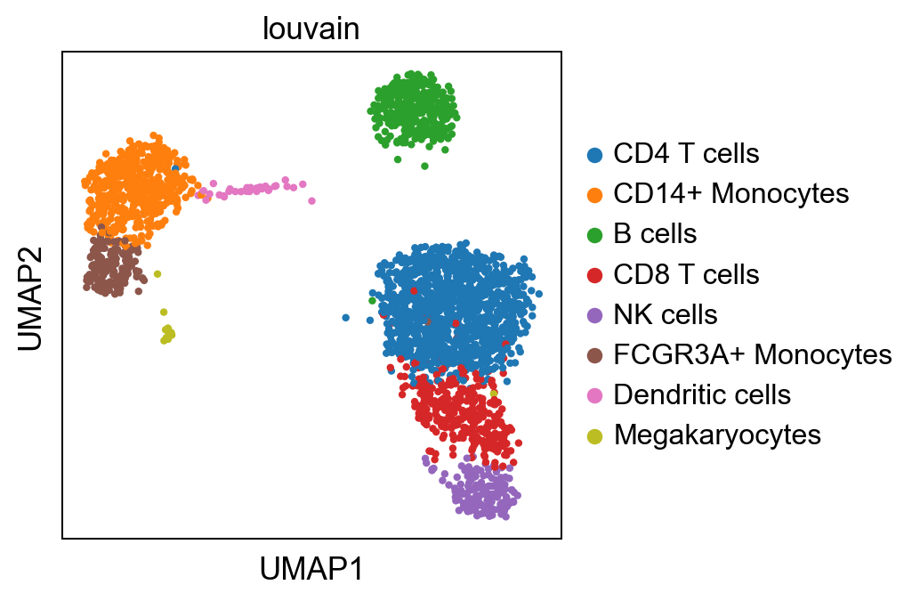
We load the human PBMC data available from scanpy.

[2]:

adata = sc.datasets.pbmc3k_processed()
adata

[2]:

AnnData object with n_obs × n_vars = 2638 × 1838
    obs: 'n_genes', 'percent_mito', 'n_counts', 'louvain'
    var: 'n_cells'
    uns: 'draw_graph', 'louvain', 'louvain_colors', 'neighbors', 'pca', 'rank_genes_groups'
    obsm: 'X_pca', 'X_tsne', 'X_umap', 'X_draw_graph_fr'
    varm: 'PCs'
    obsp: 'distances', 'connectivities'

[3]:

sc.pl.umap(adata, color="louvain")

/Users/diez/miniconda3/envs/singleCellHaystack/lib/python3.10/site-packages/scanpy/plotting/_tools/scatterplots.py:392: UserWarning: No data for colormapping provided via 'c'. Parameters 'cmap' will be ignored
  cax = scatter(

Filter some cells#

We remove Megakaryocytes since they are not interesting in this example and they will drive the top results.

[4]:

mega = adata.obs.louvain.isin(["Megakaryocytes"])
mega.value_counts()

[4]:

False    2623
True       15
Name: louvain, dtype: int64

[5]:

adata = adata[~mega, :]
adata

[5]:

View of AnnData object with n_obs × n_vars = 2623 × 1838
    obs: 'n_genes', 'percent_mito', 'n_counts', 'louvain'
    var: 'n_cells'
    uns: 'draw_graph', 'louvain', 'louvain_colors', 'neighbors', 'pca', 'rank_genes_groups'
    obsm: 'X_pca', 'X_tsne', 'X_umap', 'X_draw_graph_fr'
    varm: 'PCs'
    obsp: 'distances', 'connectivities'

Run haystack#

We run haystack using PCA coordinates and otherwise default parameters. Since the data has been scaled, we need to pass the raw data to avoid negative numbers. Also this will allow haystack to run on all the genes, not only those to calculate the PCA coordinates.

[6]:

res = hs.haystack(adata.raw.to_adata(), coord="pca")

> starting haystack ...
> entering array method ...
> scaling coordinates ...
> calculating feature stds ...
> removing 6 genes with zero variance ...
> calculating grid points ...
> calculating distance to cells ...
> calculating densities ...
> calculating Q dist ...
> calculating KLD for 13708 features ...

100%|██████████| 13708/13708 [00:02<00:00, 6130.26it/s]

> calculating feature's CV ...
> selecting genes to randomize ...
> calculating randomized KLD ...

100%|██████████| 100/100 [00:02<00:00, 40.36it/s]

> calculating P values ...
> done.

Check some QC plots#

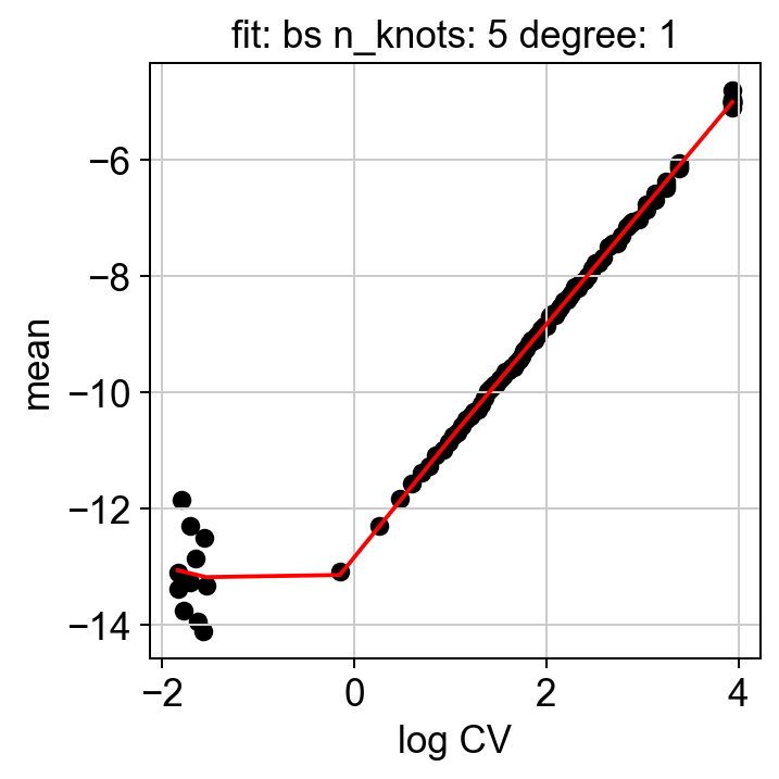
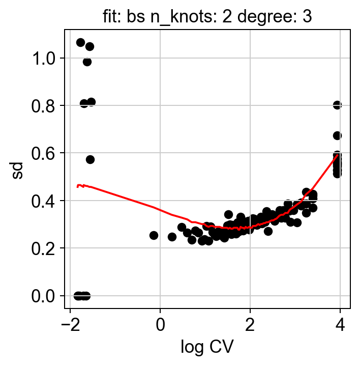
We can examine some of the QC plots. First the randomization fits. These are used to calculate KLD from randomized expression levels for a subset of genes, in order to estimate the values to the entire gene set.

[7]:

hs.plot_rand_fit(res, "mean")
hs.plot_rand_fit(res, "sd")

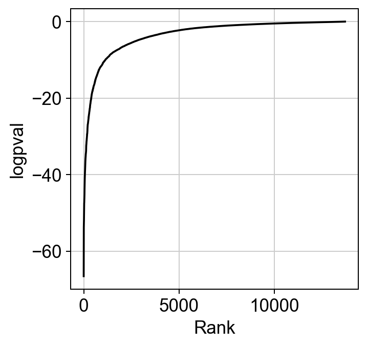
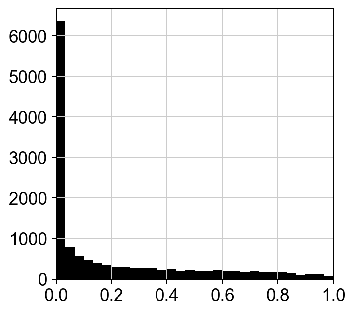
The ranking of logpval and distribution of pval gives us some idea of how many significant genes we can detect.

[8]:

hs.plot_pval_rank(res)
hs.plot_pval_hist(res)

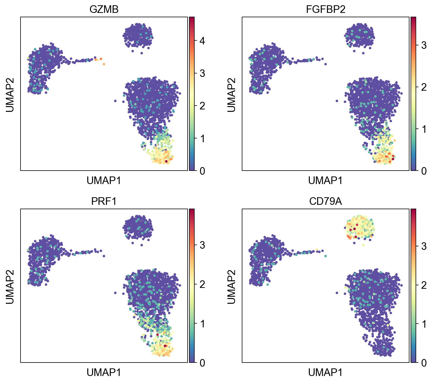
Visualizing the results#

A pandas DataFrame with the results can be obtained. By default the results are sorted by logpval_adj.

[9]:

sum = res.top_features(n=10)
sum

[9]:

	gene	KLD	pval	pval_adj	logpval	logpval_adj
9290	GZMB	0.004207	2.671463e-67	3.662041e-63	-66.573251	-62.436277
3200	FGFBP2	0.003713	2.990241e-63	4.099023e-59	-62.524294	-58.387320
7149	PRF1	0.002337	2.624538e-57	3.597716e-53	-56.580947	-52.443973
12799	CD79A	0.002090	1.626349e-56	2.229399e-52	-55.788786	-51.651812
1802	GNLY	0.002155	3.416672e-56	4.683574e-52	-55.466397	-51.329423
...	...	...	...	...	...	...
13172	A1BG-AS1	0.000098	9.969061e-01	1.000000e+00	-0.001346	0.000000
344	SYNC	0.000088	9.974878e-01	1.000000e+00	-0.001092	0.000000
1731	PCYOX1	0.000065	9.980668e-01	1.000000e+00	-0.000840	0.000000
13247	CRKL	0.000038	9.988439e-01	1.000000e+00	-0.000502	0.000000
9925	STOML1	0.000099	9.989249e-01	1.000000e+00	-0.000467	0.000000

13708 rows × 6 columns

[10]:

sc.pl.umap(adata, color=sum.gene.iloc[:4], ncols=2, cmap="Spectral_r")

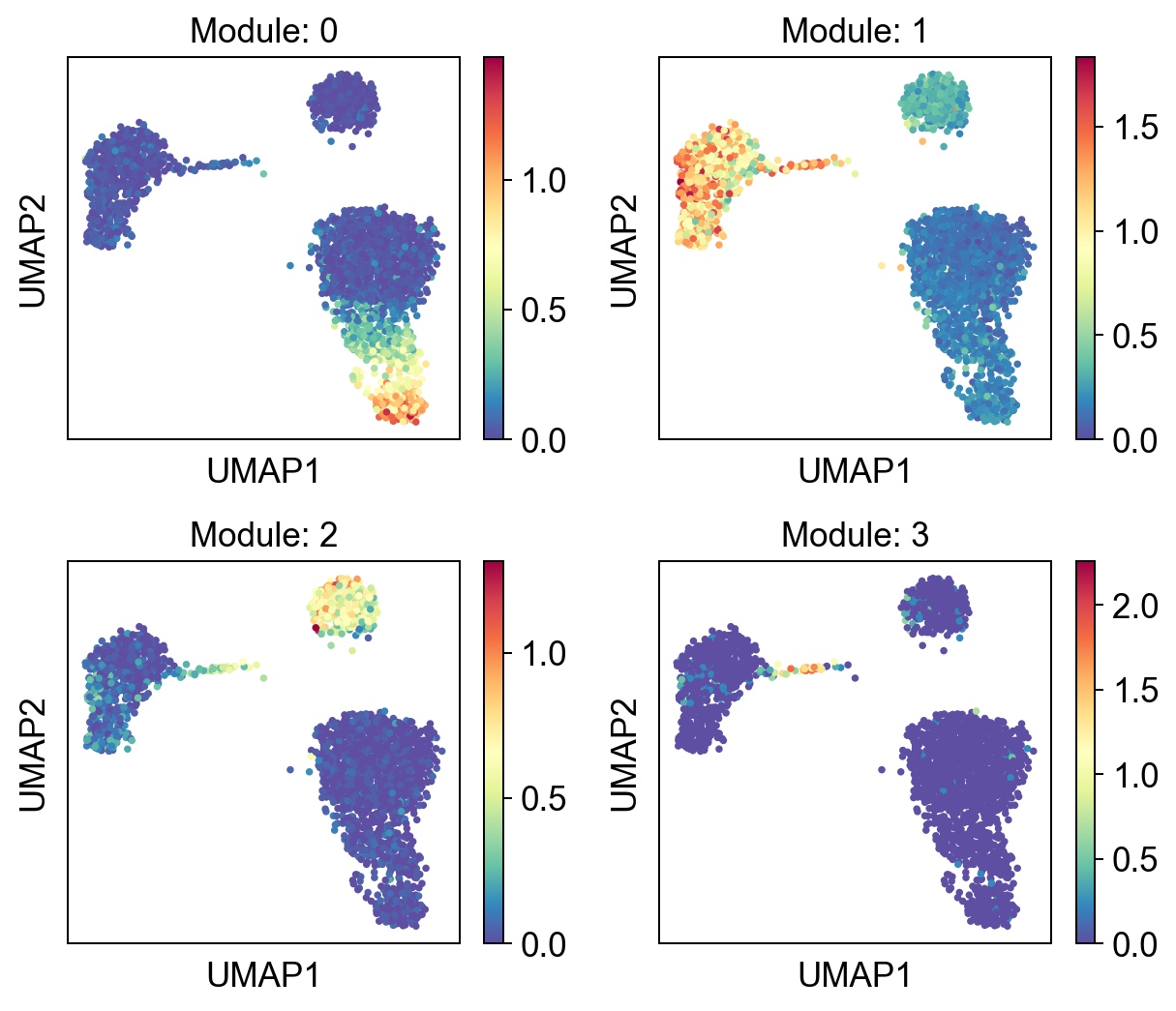
Clustering results into gene modules#

We can cluster the results using K-means. We need to pass the AnnData object, the haystack results and the number of clusters.

[11]:

gene_mods = hs.cluster_genes(adata.raw.to_adata(), res, n_clusters=4, random_state=1)
gene_mods.sort_values("cluster").groupby("cluster").head(3)

[11]:

	gene	cluster
0	GZMB	0
48	CCL5	0
46	CTSW	0
63	CEBPD	1
64	SPI1	1
71	NCF2	1
3	CD79A	2
96	PKIG	2
11	HLA-DQA1	2
61	CD1C	3
6	FCER1A	3
20	CLEC10A	3

[12]:

hs.plot_gene_clusters(adata.raw.to_adata(), gene_mods, basis="umap", ncols=2, figsize=[7, 6],   color_map="Spectral_r")

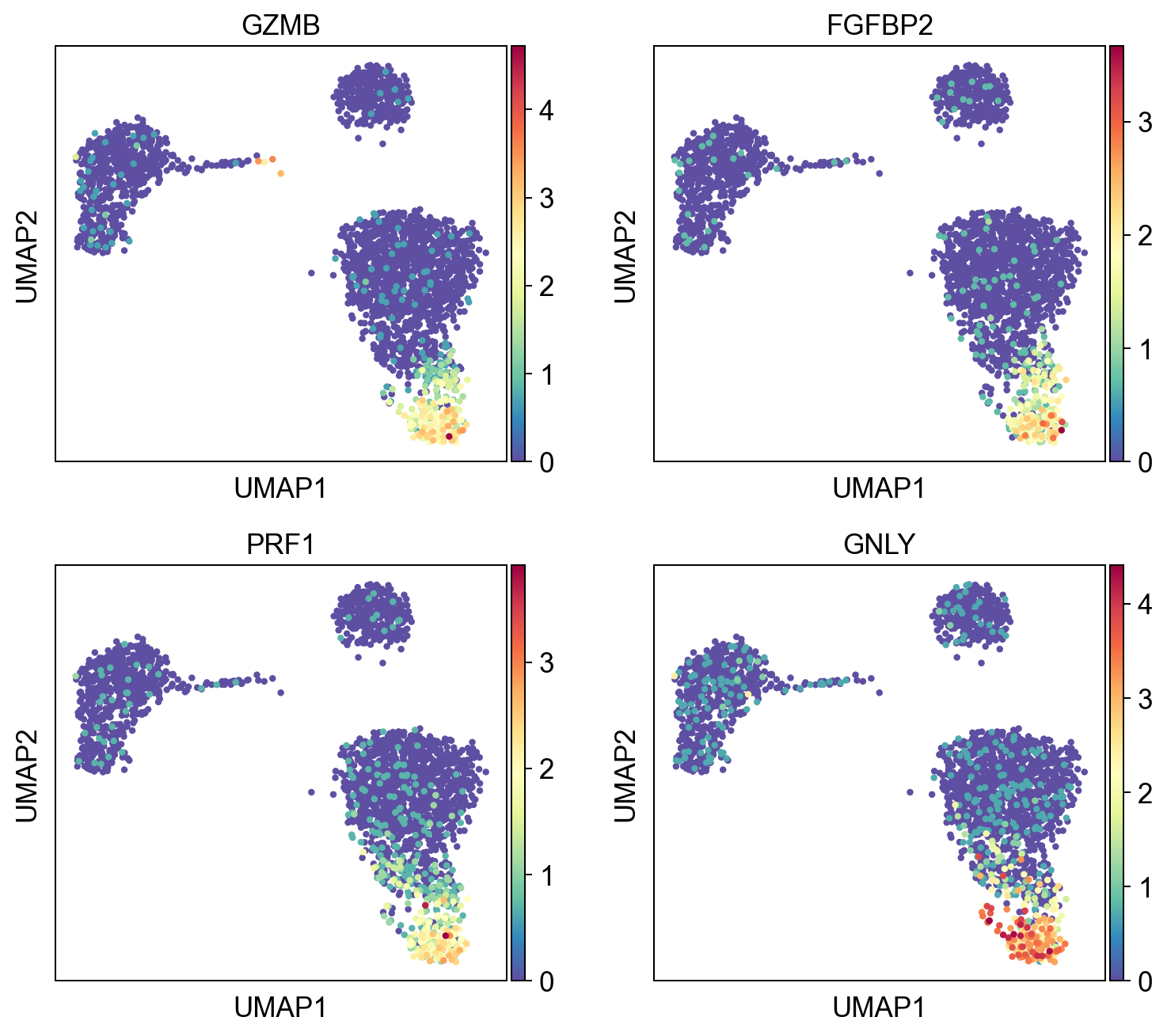
Check some of the genes in Module 0.

[13]:

mod0 = gene_mods.groupby("cluster").get_group(0)
mod0.head(4)

[13]:

	gene	cluster
0	GZMB	0
1	FGFBP2	0
2	PRF1	0
4	GNLY	0

[14]:

sc.pl.umap(adata, color=mod0.gene.iloc[:4], cmap="Spectral_r", ncols=2)

Export results#

[15]:

#sum.to_csv("pbmc3k-results.tsv")

Single Cell Transcriptomics (PBMC3k)

Contents